Human Visual System: A Quick Introduction (Part 2: Representation)

In the previous blog, we discussed the first stage of human visual system (HVS) viz. encoding. It explained how the light coming to our eyes is converted into neural signals. In this blog, we will learn about the next stage: representation.

Representation

When light hits the photoreceptors, it starts a series of chain reaction that carries information from the retina through a collection of different neurons called visual streams to the visual cortex, the part of the human brain dedicated to visual processing. Visual stream operates in parallel, and each stream specializes in analyzing different aspects of the retinal image. The segregation of streams starts with rods and cones in the retina and continues into the cortical areas. Hundreds of rods connect directly to a single bipolar cell, which connects to retinal ganglion cells in the outermost layer of the retina. In contrast, very few cones converge onto one retinal ganglion cell. This organization of neurons allows the rod pathway to be more sensitive to light at the cost of reduced acuity and the cone pathway to have higher acuity but lower sensitivity. Information is also passed laterally between retinal neurons through horizontal and amacrine cells. This complicated communication structure between retinal neurons is responsible for a significant portion of visual processing. It leads to the formation of complex receptive fields such as center-surround or on-off fields, which allows the cells to adjust their sensitivity to edges, color, and motion.

Signals from retinal ganglion cells are collected and carried by the optic nerve to the lateral geniculate nucleus (LGN) in the thalamus.

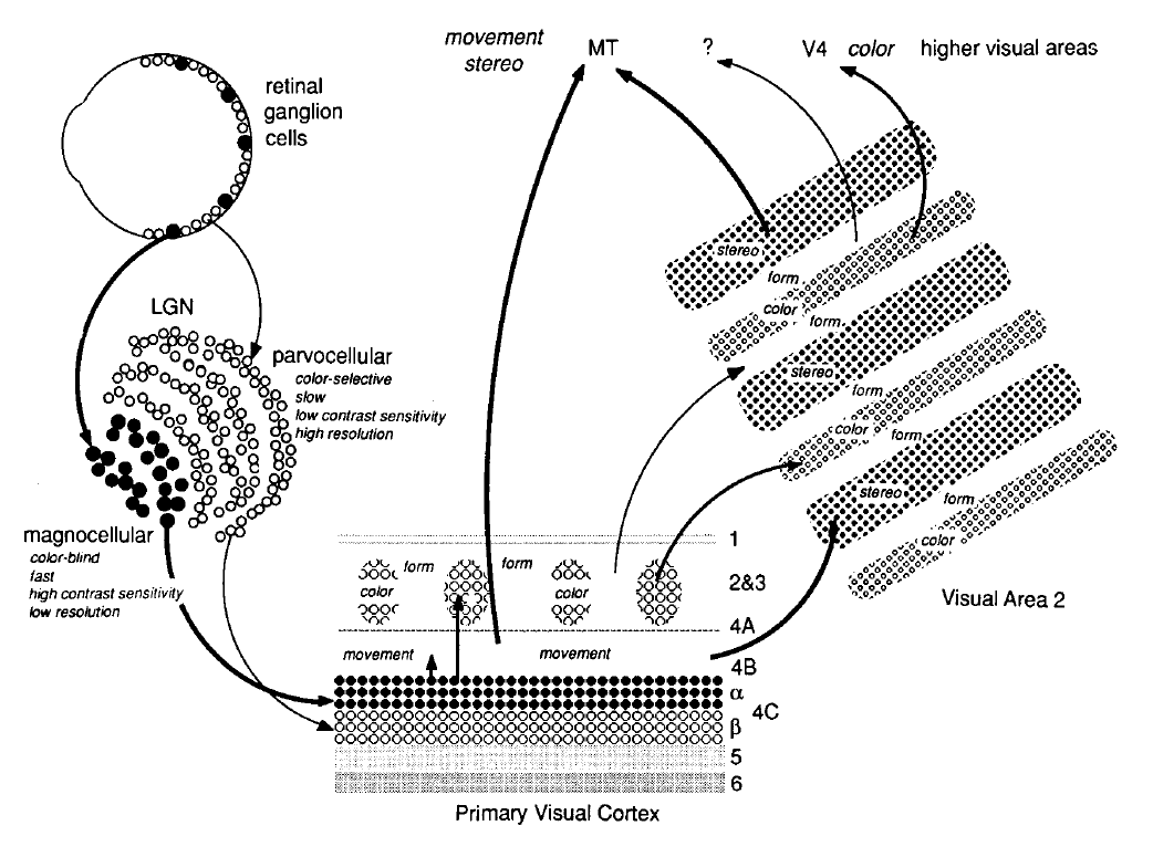
Within this pathway, two well-studied streams include parvocellular and magnocellular pathways. The parvocellular pathway connects ganglion cells to the upper layers of the LGN (P layers), containing neurons with small cell bodies. They respond to color, fine details, and still or slow moving objects. Magnocellular pathways connect ganglion cells to two deeper layers of the LGN (M layers) comprising of neurons with larger cell bodies which respond to objects in motion. These layers connect to different areas of the primary visual cortex, also called ventral area V1. Neurons in the visual cortex are more complex than retinal neurons and respond asymmetrically to different edge orientations, motion directions, and binocular disparity. Roles of different neurons are also non-uniformly distributed, with 30% of the primary visual cortex responsible for the central 5° of the visual field. At the same time, the periphery is under-represented. Neural representation becomes increasingly more complex as the information flows from the primary visual cortex through a visual hierarchy in V2, V3, V4, V5 and the visual association cortex via the dorsal and ventral streams. The neurons in the dorsal stream are involved in interpreting spatial information such as the location and motion of the objects. In contrast, neurons in the ventral stream help determine object characteristics such as color and shape. It should be noted that the visual system does not create new streams as the visual task or imaging condition changes. The visual neurons instead change their sensitivity to light stimulation in response to imaging conditions by a process called visual adaptation. One of the most salient examples of this phenomenon is luminance adaptation which decreases (or increases) the light sensitivity of individual neurons in the visual pathway in response to increasing (or decreasing) illumination levels. This extends the sensing abilities of our eyes to nine orders of magnitude, allowing us to clearly see both a dark starry sky and a bright sun. Change in sensitivity of the visual pathway aims to achieve a constant representation of image contrast instead of absolute light levels. Image contrast is the ratio of local intensity and the mean image intensity. Preserving image contrast improves our ability to distinguish objects in both very bright and dark environments.

Contrast sensitivity function

The activity of all the neurons in the HVS can be summarized by an abstract psychophysical construct called a neural image. A neural image contains all the information available to an observer after all the neural transformations have been applied to the real image. Knowledge of the neural transformations and the corresponding neural image can help us optimize how we store and display visual media. One way to determine these neural transformations is to measure the responses of all individual neurons and the connections between them. This is obviously an extremely invasive and impractical procedure. An alternate, more practical approach is to study the behavior of the visual system when presented with detection and discrimination tasks on spatio-temporal contrast patterns:

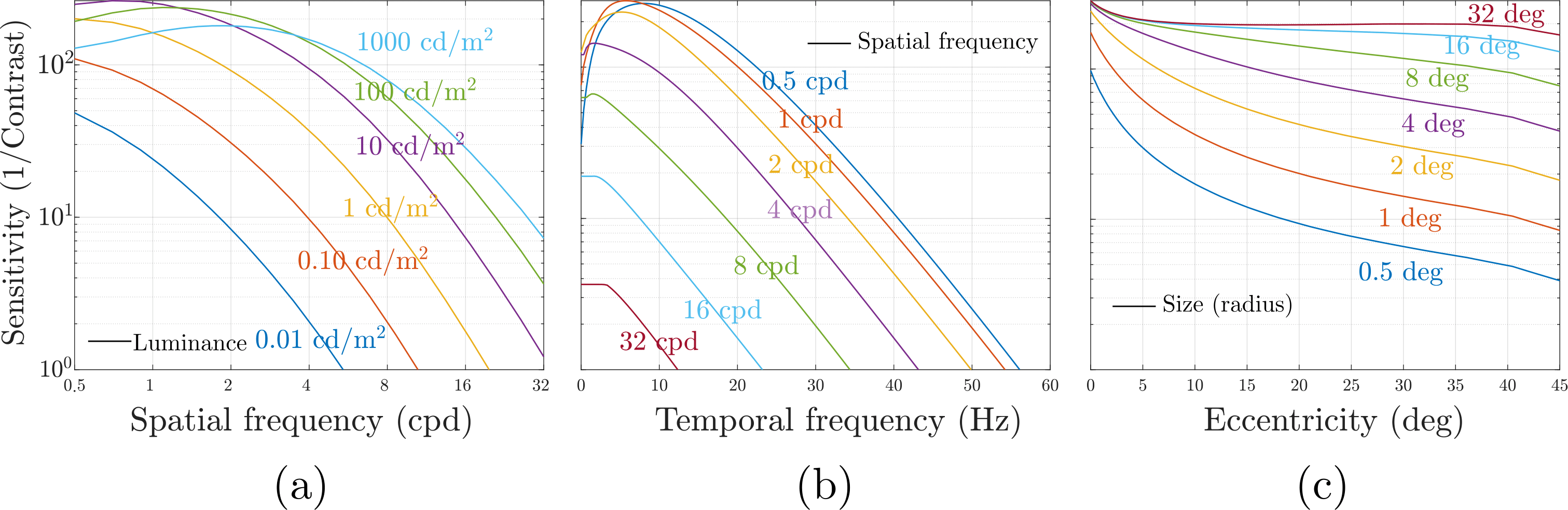
The results from these experiments are used to develop models of contrast sensitivity called contrast sensitivity functions (CSFs) that predict the magnitude of contrast necessary to detect a pattern described by the parameters of the CSF. A CSF is a high dimensional function because our perception depends on several factors such as the pattern’s spatial and temporal frequency, size, color, eccentricity, background luminance, and orientation. The figure below plots contrast sensitivity (reciprocal of contrast threshold) w.r.t. to some of these parameters. Notice how the predictions of CSF closely match the anatomy of the visual system. Our sensitivity to high spatial frequencies is drastically reduced (a), similar to the MTF of our lens. Similarly, our sensitivity rapidly goes down with increasing eccentricity (c) matching the distribution of cones on our retina. This decrease in sensitivity with eccentricity is reversed by increasing the stimulus’s size, similar to how a higher number of neurons in the visual cortex results in improved image quality (called cortical magnification). CSF also predicts our sensitivity to temporally varying (flickering) stimuli (b). The points at which the lines in the plot intersect with the x-axis (temporal frequency) are known as critical flicker frequency, and the flickering light source starts appearing to be completely steady at those points. Such measurements from the CSF are instrumental in choosing the spatial resolution and refresh rate while designing displays.

Given any real image, CSF can be used to find the corresponding neural image assuming a shift-invariant zero phase shift mapping between the two. Note that we do not have any mechanism to measure the neural image, but only the input threshold stimulus and observer’s detection threshold. Since detection is a result of increasing or decreasing neurons’ firing rate pooled over the entire neural image, we need to apply a static nonlinearity to the neural image that ignores the sign of neural responses and incorporates responses from different neurons. The exact nature of this non-linearity is a contested topic, but popular choices include sum of squares, sum of absolute values, and Minkowski norm. Due to their relative simplicity, CSFs have found many applications in image and video quality metrics, tonemapping, video compression, foveated rendering, 3D level-of-detail , variable rate shading, and other areas of computer graphics.